LaneKerbNet Algorithm

1. Introduction

To tackle the limitation of traditional methods for lane and curb detection, the features should be learned automatically with deep neural networks instead of modeling hand-crafted feature descriptors. Since bounding box is not suitable for detecting long continuous objects, most popular approaches relying on object proposals and classification step like Mask R-CNN 1 can not perform well for lane and curb instance segmentation. Inspired by the semantic segmentation network and instance segmentation task based on distance metric learning 3, a two-branch network is designed. Besides the commonly used pixel-wise softmax loss in semantic segmentation, another equally important discriminative loss is introduced, which can enforce the curb points of the same instance lie close together in the pixel embedded N-dimensional feature space and those belong to different instances lie far apart. Therefore, the trained two-branch network can output different clusters automatically with simple post-processing. And it can also cope with arbitrary number of lane and curb instances.

The off-the-shelf architecture FCN-8s is used for semantic segmentation. In our framework, the end-to-end lane and curb instance segmentation does not require too much changes on the backbone network.

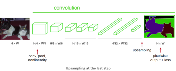
Fig. 6 Semantic segmentation.

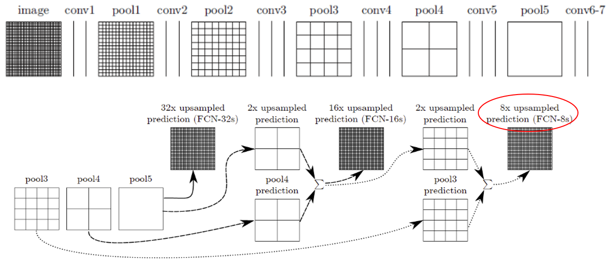
Fig. 7 FCN-8s.

2. Method

Given an input image, the goal is to obtain where is the lane and curb location and how many lane and curb instances exist in the image.

2.1 Network Architecture

The multi-lane and multi-curb detection problem is addressed under the fully convolutional network architecture. LaneKerbNet’s network architecture consists of typical encoder-decoder network 2, and then followed by a two-branched network which are class segmentation branch and pixel embedding branch as shown in Fig. 8. The output of first branch is a two channel image, and the output of second branch is a N channel image (N is the pixel embedding dimension). The loss function \(Loss\) is designed combining equally weighted class segmentation loss \(loss_b\) and pixel embedding discriminative loss \(loss_p\), which is shown in (3) will be described in details later.

(3)\[\begin{equation} Loss = 0.5loss_b + 0.5loss_p \end{equation}\]

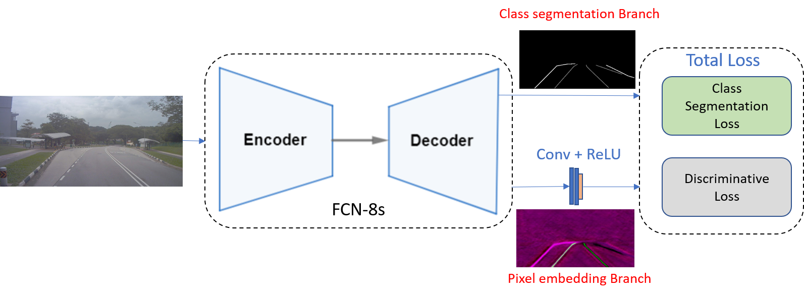
Fig. 8 Lanekerbnet network architecture.

2.1.1 Class Segmentation Branch

The class segmentation branch is trained to produce a two class segmentation map predicting which pixels is lane and curb and the remaining pixels belong to background. To construct the lane and curb ground truth labels, the ground-truth lane or curb points are connected to form a connected line per lane or per curb. The lane and curb labels are then drew with thickness 5 on each lane and curb line. The class segmentation use 255 to represent the lane field, 127 to represent the curb field and 0 for the rest. The loss function of class segmentation branch is the sparse softmax cross entropy loss function defined as:

(4)\[\begin{equation} softmax(logits_{i}) = \frac{e^{logits_{i}}}{\sum_{i}^{n}e^{logits_{i}}} \end{equation}\]

(5)\[\begin{equation} loss_{b} = - \sum_{i}^{n} y_{i}\ln{(softmax(logits_{i}))} \end{equation}\]

where \(n\) is the class number. \(y_i\) is the ith class label. \(logits_i\) is the last layer output of the class segmentation branch. \(softmax(logits_{i})\) is to produce the probability of assigning to one class.

Since the lane, curb and background pixel numbers are highly unbalanced, we used a custom class weighting scheme defined as:

(6)\[\begin{equation} w_{class_{i}} = \frac{1}{\ln{(c+p_{class_{i}})}} \end{equation}\]

(7)\[\begin{equation} p_{class_{i}} = \frac{cout_{class_{i}}}{\sum_{i}^{n}cout_{class_{i}}} \end{equation}\]

where \(c\) is a hyper-parameter, which we set to 1.02. Thus, the weights \(w_{class_i}\) are bounded in the interval of [1, 50].

2.1.2 Pixel Embedding Branch

To cluster the lane and curb pixels output from the class segmentation branch, we design a pixel embedding branch for curb instance segmentation. Pixel embedding is to map each lane and curb pixel to a vector in N-dimensional feature space. We train the branch to make the intra cluster distance minimized and inter cluster distance maximized in N-dimensional feature space. Hence, the pixel embeddings belonging to the same lane or curb will be clustered together as a lane or curb instance when testing a new input image.

The pixel embedding discriminative loss lossp consisting of three terms is now introduced:

Fig. 9 Intra cluster distance minimized and inter cluster distance maximized.

• Variance term (\(L_{var}\)): a pull force that pull pixel embedding towards the mean embedding of the same lane and curb.

• Distance term (\(L_{dist}\)): a push force that push the mean pixel embedding of different lanes and curbs away from each other.

• Regularization term (\(L_{reg}\)): a force that draw all the cluster center towards the origin.

(8)\[\begin{equation} L_{var} = \frac{1}{C}\sum_{c=1}^{C}\frac{1}{N_{c}}[||\mu_{c}-x_{i}||-r_{v}]_{+}^{2} \end{equation}\]

(9)\[\begin{equation} L_{dist} = \frac{1}{C(C-1)}\sum_{c_{a}=1}^{C}\sum_{c_{b}=1,c_{a}\neq c_{b} }^{C}[||\mu_{c_{a}}-\mu_{c_{b}}||-2r_{d}]_{+}^{2} \end{equation}\]

(10)\[\begin{equation} L_{reg} = \frac{1}{C}\sum_{c=1}^{C}||\mu_{c}|| \end{equation}\]

(11)\[\begin{equation} loss_{p} = \alpha \cdot L_{var} + \beta \cdot L_{dist} + \gamma \cdot L_{reg} \end{equation}\]

where \(C\) is the number of lanes and curbs (clusters), \(N_c\) is the cluster \(c\) pixel number, \(x_i\) is the pixel embedding in the feature space, \(\mu_{c}\) is the mean value, ||·|| is the L2 norm, and \([x]_{+}= \max(0,x)\) which means that the pull force will only be activated when the pixel embedding is further from the \(r_v\) of its cluster center and the two cluster centers will be pushed away when they are closer than \(2r_d\). \(\alpha =1, \beta = 1, \gamma = 0.001\) in our experiments. The pixel embedding branch is trained so that the each lane and curb instance will be grouped together (smaller than \(r_v\)) in the pixel embedding feature space, and different lanes and curbs are lay further than \(2r_d\) from each other in the pixel embedding feature space.

2.1.3 Lane and Curb Instance Clustering

The class segmentation branch output is adopted as a mask to obtain the pixel embedding feature space values rather than directly perform pixel embedding clustering. If we set \(r_{d} > 6r_{c}\) in the above training \(loss_{p}\), then during inference, we can randomly select an unlabeled pixel embedding and apply threshold around its embedding with radius of \(2r_{c}\) to group all lane and curb pixels belonging to the same instance. Then we update the mean pixel embedding and use the new mean to threshold again by applying mean-shift algorithm 4 until mean convergence. Another pixel without assigning label will be selected to repeat the whole process until all pixels are labeled.

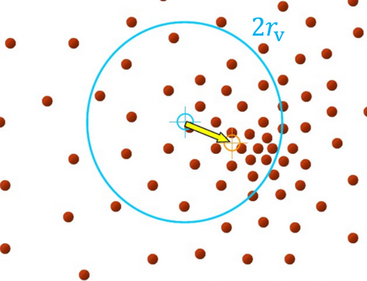
Fig. 10 Illustration of clustering process.

3. Experiments

The image resolution is resized to \(512\times256\). The embedding dimension is 4 and \(r_{v}=0.5, r_{d}=3\) in the experiments. LaneKerbNet is trained with hyper parameters batch size = 8 and learning rate \(5\mathrm{e}{-4}\). The loss is minimized by stochastic gradient descent (SGD).

We have tested our lane and curb detection algorithm with resolution of \(512\times256\). The platform is on a normal PC with Nvidia GeForec GTX 1080, Intel(R) Core i7-4770 CPU @ 3.40GHz \(\times\) 8 and 8 GB RAM. The processing speed is fast and can reach around 30 frames per second (fps). The training accuracy is about 95% on the collected rosbag data on bus.

1

J. Dai, K. He, and J. Sun, “Instance-aware semantic segmentation via multi-task network cascades,” in Proceedings of the IEEE Conference on Computer Vision and Pattern Recognition, pp. 3150-3158, 2016.

2

J. Long, E. Shelhamer, and T. Darrell, “Fully convolutional networks for semantic segmentation,” in Proceedings of the IEEE conference on computer vision and pattern recognition, pp. 3431-3440, 2015.

3

B. De Brabandere, D. Neven, and L. Van Gool, “Semantic instance segmentation with a discriminative loss function,” arXiv preprint arXiv:1708.02551, 2017.

4

K. Fukunaga and L. Hostetler, “The estimation of the gradient of a density function, with applications in pattern recognition,” IEEE Transactions on information theory, vol. 21, no. 1, pp. 32-40, 1975.